Deep learning with point clouds
Over the last decade, there have been outstanding progress in the field of 2D vision on tasks such as image classification, object detection or semantic segementation. There are several factors that contributed to these breakthroughs among which the availability of large annotated datasets or the advent of GPUs for numerical computation. But we can argue that the convolutional neural networks (CNNs) were what really changed the landscape of computer vision.
Advanced robotic systems, such as a self-driving car, generally require visual perception capabilities beyond 2D images. 3D data generated by 3D scanners often come in the format of point clouds, an unordered set of 3D points, and therefore invariant to permutations of its members. Due to this property, convolving kernels with point clouds cannot be done as it is for 2D images.
In this article we will review the challenges associated with learning features from point clouds. We will also go through a detailed analysis of PointNet, the deep learning pioneer architecture for point clouds. A PyTorch implementation of PointNet will be proposed. Finally we will review the limits of PointNet and have a quick overview of the proposed solutions to these limits.
Point clouds
A point cloud is simply an unordered set of 3D points, and might be accompanied by features such as RGB or intensity.
| X | Y | Z |
| 0.07388 | 0.16975 | -0.19326 |
| 0.15286 | 0.15050 | 0.24355 |
| 0.20948 | 0.15050 | 0.29081 |
| ... | ... | ... |
By nature, point clouds are irregular (with regard to their density) and unordered, and therefore invariant to permutations of their members. There are many ways to visualize point clouds among which the open3d python library.
import open3d

pcd = open3d.read_point_cloud('point_cloud_data.txt')
open3d.draw_geometries([pcd])
This should open a 3D visualization similar to the image below for which the point cloud is a sample of the ShapeNet dataset. There are some other available datasets such as the Semantic3D dataset or the S3DIS dataset.
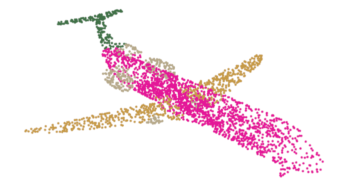
Fig. 1: Point cloud visualization with Open3D.
Another great alternative for point cloud visualization is CloudCompare, an open source software which comes with a graphical user interface among other tools.
A point cloud is not the only available representation for 3D data. Among others, the voxel[1] and the multi-views[2] approaches are worth discussing here. As 2D images are represented as grids of pixels, a 3D object/scene could also be mapped to a grid of voxels (the 3D equivalent of a pixel). This representation has a great advantage: most of the techniques developed for regular domain data such as images can be applied to it. But this volumetric representation is limited by its computation (and storage) cost, and also by its resolution due to data sparsity. On the other hand, there is even a more direct way to leverage regular domain techniques: using 2D images of an object/scene taken from different viewpoint. This is the so called multi-views approach. Although it has achieved great performance on classification, it is not that easy to extend this to point semantic segmentation or scene understanding. Both these two alternative approaches leverage the power of the convolution operation which will be quickly explained in the next section. Unfortunately, a point cloud being an unordered set of points, it is impossible to direclty convolve a kernel with it. In the next section, this problem is going to be illustrated.
Problem statement
As previously mentionned, the convolution operation is one of the key contributors to the 2D vision performance of neural networks. The fundamental building block of a CNN is illustrated below.
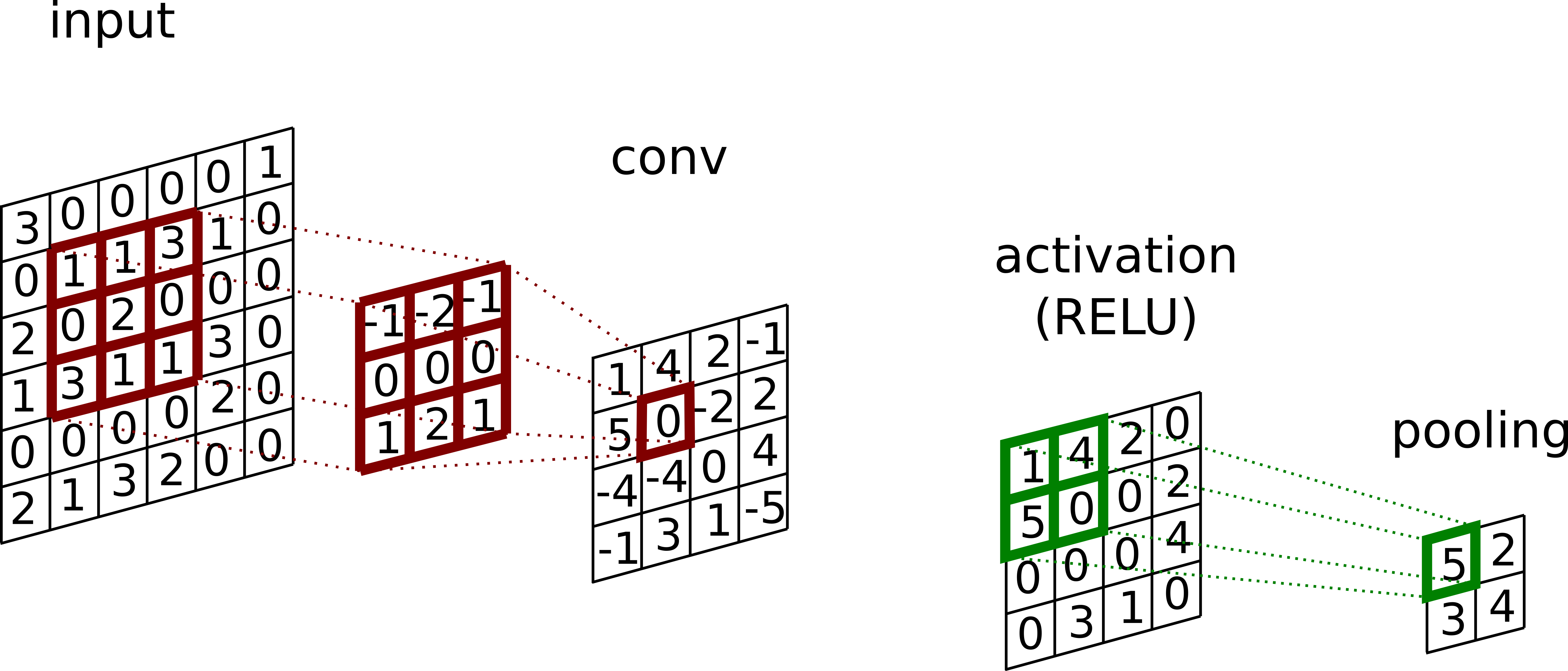
Fig. 2: The convolution block.
A kernel is first convolved with the input, then a non linear activation function (e.g. RELU) is applied, and finally a pooling (e.g. max) is performed to produce the so called feature map. Generally there are several kernels applied per block resulting in several feature maps.
The convolution operation leverages 3 key ideas:
- Sparse connectivity: by making the kernel size k smaller than the input size m, the algorithm runtime is
faster . Since k is generally several order of magnitude smaller than m, the gain is consequent.
- Parameter sharing: each parameter of a kernel is used at every position of the inputs. Although not decreasing the runtime, it reduces the storage requirement of the model and decouples the number of parameters from the input dimension.
- Equivariance to translation: the parameter sharing property of the convolution operation also induces the equivariance to translation property.
In addition, the use of max pooling allows the model to be invariant to small translations, and also improves the computational efficiency since the next block is going to be fed with a smaller input. The representation power of CNNs truly shines when these layers (blocks) are stacked after each other. Basically, the first convolutional layers learn low level features such as edges while the last layers learn higher level features. This is pretty much illustrated in the figure below taken from [3] where the authors used a deconvnet to visualize the activation of convolutional layers.
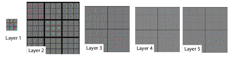
Fig. 3: Visualization of convolution layer activations (from [3]).
Naturally, we would like to apply the representation power of this simple CNN building block to point clouds. Unfortunately, doing so would result in two big problems: variance to ordering and desertion of shape.
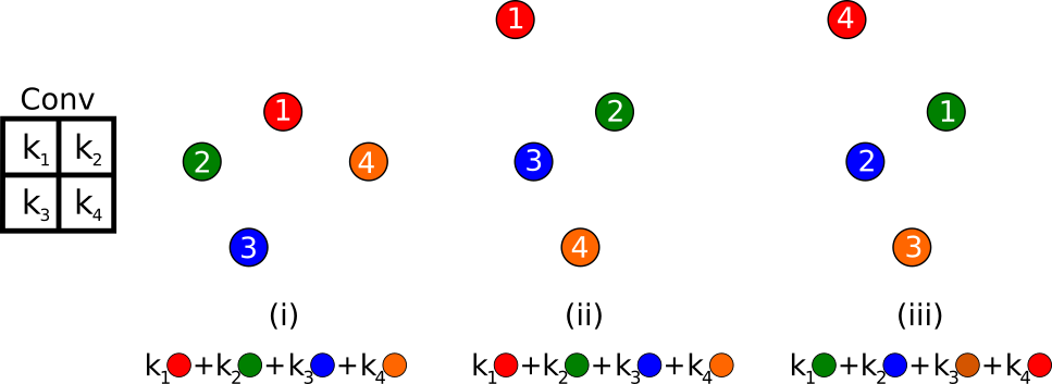
Fig. 4: Point cloud problem statement.
To illustrate these problems, let's consider the three point clouds (i, ii, iii) in the image above. Each of them is made of 4 points, and each of these points has a feature associated with itself, represented here by the color of the point. Consider now that we would like to convolve a kernel with these point clouds. The convolution relative ordering considered here is represented by the number associated with the points. Doing so, we would get :
Having results in a desertion of shape (the shape of the cloud (i) is clearly different than the shape of the cloud (ii)). In addition
while the cloud shape and features are identical means that the convolution operation would lead to a variance to ordering.
This example illustrates clearly why we can't simply convolve kernerls with point clouds like it is done for data represented in regular domains such as images. It also defines pretty well the problem associated with learning features from point clouds. We need to find a function to replace the convolution operation and this function must exhibit the following properties:
- Invariance to permutations: in the example above, that means that
. More generally, a function f of N variables
is said to be invariant under permutations if the value of f does not change under permutations of its variables. For N=3, this means
- Sensitive to the local structure induced by the distance metric: from the example above, this would mean
- Invariance to geometric transformations such as rotations or translations of the whole point set.
This problem of permutation invariance is not really specific to point clouds, but it rather forms a general problem associated with sets. A more generic approach for this problem can be found in the "Deep sets" paper [4]. In addition I found this blog article [5] particularly instructive on this topic.
PointNet
The first proposal to solve the aforementioned problem is PointNet[6], a paper published at CVPR 2017. Their approach is somewhat simple:
- A shared MLP (multi layer perceptron) allows for learning a spatial encoding for each point.
- A max pooling function is used as a symmetric function to solve the invariance to permutation issue. It destroys the ordering information and makes the model permutation invariant.
- Finally to make the model resilient to geometric transformation such as rotations or translation of the whole point set, alignment networks are used to learn transformation matrices. These matrices somehow align their inputs to a canonical space, and are similar to the spatial transformer network introduced by Jadeberg[7] for 2D images.
The authors formally demonstrate in the paper that a max pooling function associated with the learned spatial encoding of each point can be used as a general function approximator. In the worst case, the network can learn to convert the input points into a volumetric representation, but in practice the network is able to learn a better representation of the input data.
The full PointNet architecture can be visualized in the image below taken from the original paper. In order to gain a deeper understanding of it, we will go through a step by step PyTorch implementation. The full code can be found on this GitHub repository.
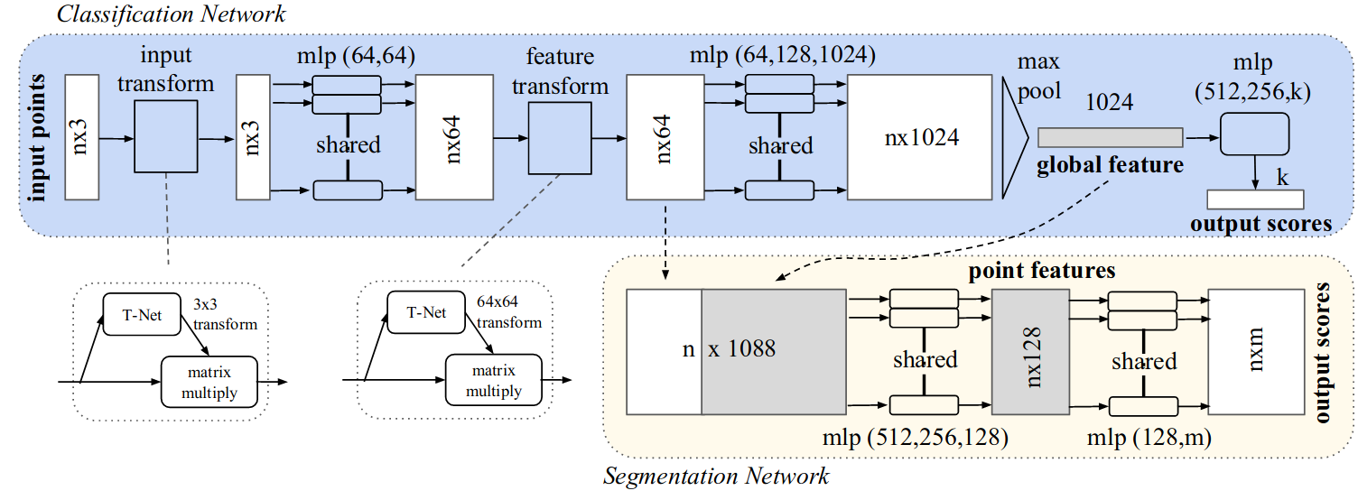
Fig. 5: PointNet architecture (from [6])
We will start by defining the transformation networks (input and feature transform). They are in part very similar to the full PointNet:
- A shared MLP is used to learn a spatial encoding for each point. These shared MLP can be identically implemented here by using a 1D convolution with a kernel size 1.
- A max pooling operation to gather the global information.
- Fully connected layers are used to project the result of the max pooling to the expected matrix dimensions.
The implementation given below can be used both for the input and feature transforms simply by specifying the expected output dimension (respectively 3 and 64).
import torch
import torch.nn as nn
import torch.nn.functional as F


class TransformationNet(nn.Module):

    def __init__(self, input_dim, output_dim):
        super(TransformationNet, self).__init__()
        self.output_dim = output_dim

        self.conv_1 = nn.Conv1d(input_dim, 64, 1)
        self.conv_2 = nn.Conv1d(64, 128, 1)
        self.conv_3 = nn.Conv1d(128, 1024, 1)

        self.bn_1 = nn.BatchNorm1d(64)
        self.bn_2 = nn.BatchNorm1d(128)
        self.bn_3 = nn.BatchNorm1d(1024)
        self.bn_4 = nn.BatchNorm1d(512)
        self.bn_5 = nn.BatchNorm1d(256)

        self.fc_1 = nn.Linear(1024, 512)
        self.fc_2 = nn.Linear(512, 256)
        self.fc_3 = nn.Linear(256, self.output_dim*self.output_dim)

    def forward(self, x):
        num_points = x.shape[1]
        x = x.transpose(2, 1)
        x = F.relu(self.bn_1(self.conv_1(x)))
        x = F.relu(self.bn_2(self.conv_2(x)))
        x = F.relu(self.bn_3(self.conv_3(x)))

        x = nn.MaxPool1d(num_points)(x)
        x = x.view(-1, 1024)

        x = F.relu(self.bn_4(self.fc_1(x)))
        x = F.relu(self.bn_5(self.fc_2(x)))
        x = self.fc_3(x)

        identity_matrix = torch.eye(self.output_dim)
        if torch.cuda.is_available():
            identity_matrix = identity_matrix.cuda()
        x = x.view(-1, self.output_dim, self.output_dim) + identity_matrix
        return x
The PointNet architecture can be used both for classification and semantic segmentation. We will define a base structure which can therefore be extended for each task. This base module includes two transformation networks as defined above, but also the point encoding and the max pooling operation. Again point encoding is done via a shared MLP that can be replaced in the implementation by a 1D convolution operation with a kernel size 1. There are eventually a couple of details important to notice:
- The semantic segmentation task needs some local features in order to perform well. Therefore the local features (output of the feature transform) are combined with the ouput of the max pooling operation. In the implementation below, the flag return_local_features allows for this combination.
- As you can notice, the output of this BasePointNet also contained the feature_transform matrix. According to the orignal paper, some optimization problems can be encountered due to its size (64*64). Therefore they add a regulation term to the loss to force this matrix to be closed to orthogonal:
where I is the identity matrix and A is the feature transform matrix.
class BasePointNet(nn.Module):

    def __init__(self, point_dimension, return_local_features=False):
        super(BasePointNet, self).__init__()
        self.return_local_features = return_local_features
        self.input_transform = TransformationNet(input_dim=point_dimension, output_dim=point_dimension)
        self.feature_transform = TransformationNet(input_dim=64, output_dim=64)

        self.conv_1 = nn.Conv1d(point_dimension, 64, 1)
        self.conv_2 = nn.Conv1d(64, 64, 1)
        self.conv_3 = nn.Conv1d(64, 64, 1)
        self.conv_4 = nn.Conv1d(64, 128, 1)
        self.conv_5 = nn.Conv1d(128, 1024, 1)

        self.bn_1 = nn.BatchNorm1d(64)
        self.bn_2 = nn.BatchNorm1d(64)
        self.bn_3 = nn.BatchNorm1d(64)
        self.bn_4 = nn.BatchNorm1d(128)
        self.bn_5 = nn.BatchNorm1d(1024)

    def forward(self, x):
        num_points = x.shape[1]

        input_transform = self.input_transform(x)

        x = torch.bmm(x, input_transform)
        x = x.transpose(2, 1)
        x = F.relu(self.bn_1(self.conv_1(x)))
        x = F.relu(self.bn_2(self.conv_2(x)))
        x = x.transpose(2, 1)

        feature_transform = self.feature_transform(x)

        x = torch.bmm(x, feature_transform)
        local_point_features = x

        x = x.transpose(2, 1)
        x = F.relu(self.bn_3(self.conv_3(x)))
        x = F.relu(self.bn_4(self.conv_4(x)))
        x = F.relu(self.bn_5(self.conv_5(x)))
        x = nn.MaxPool1d(num_points)(x)
        x = x.view(-1, 1024)

        if self.return_local_features:
            x = x.view(-1, 1024, 1).repeat(1, 1, num_points)
            return torch.cat([x.transpose(2, 1), local_point_features], 2), feature_transform
        else:
            return x, feature_transform
Finally, as stated earlier, depending on the task (classification or segmentation), two modules are implemented. They both extend the BasePointNet module defined above.
- In the case of classification, the output of the base module is fed to a fully connected network with a softmax activation on the last layer. As in the original paper, a dropout of 0.3 is applied to the first two fully connected layers.
- For semantic segmentation, as explained above, a combination of global and local features is used. This combination is fed to some shared MLP layers (again here 1D convolutions are used). The output is then passed though a softmax for classifying any single points.
class ClassificationPointNet(nn.Module):

    def __init__(self, num_classes, dropout=0.3, point_dimension=3):
        super(ClassificationPointNet, self).__init__()
        self.base_pointnet = BasePointNet(return_local_features=False, point_dimension=point_dimension)

        self.fc_1 = nn.Linear(1024, 512)
        self.fc_2 = nn.Linear(512, 256)
        self.fc_3 = nn.Linear(256, num_classes)

        self.bn_1 = nn.BatchNorm1d(512)
        self.bn_2 = nn.BatchNorm1d(256)

        self.dropout_1 = nn.Dropout(dropout)

    def forward(self, x):
        x, feature_transform = self.base_pointnet(x)

        x = F.relu(self.bn_1(self.fc_1(x)))
        x = F.relu(self.bn_2(self.fc_2(x)))
        x = self.dropout_1(x)

        return F.log_softmax(self.fc_3(x), dim=1), feature_transform


class SegmentationPointNet(nn.Module):

    def __init__(self, num_classes, point_dimension=3):
        super(SegmentationPointNet, self).__init__()
        self.base_pointnet = BasePointNet(return_local_features=True, point_dimension=point_dimension)

        self.conv_1 = nn.Conv1d(1088, 512, 1)
        self.conv_2 = nn.Conv1d(512, 256, 1)
        self.conv_3 = nn.Conv1d(256, 128, 1)
        self.conv_4 = nn.Conv1d(128, num_classes, 1)

        self.bn_1 = nn.BatchNorm1d(512)
        self.bn_2 = nn.BatchNorm1d(256)
        self.bn_3 = nn.BatchNorm1d(128)

    def forward(self, x):
        x, feature_transform = self.base_pointnet(x)

        x = x.transpose(2, 1)
        x = F.relu(self.bn_1(self.conv_1(x)))
        x = F.relu(self.bn_2(self.conv_2(x)))
        x = F.relu(self.bn_3(self.conv_3(x)))

        x = self.conv_4(x)
        x = x.transpose(2, 1)

return F.log_softmax(x, dim=-1), feature_transform
As we can see above, the implementation of the model is pretty straight forward in PyTorch. On the GitHub repository, the full implementation, including training loop and inference can be found. Two datasets are available:
- Shapenet: Dataset made of 16 different single object classes. Each object contains several parts (up to 6) that can be segmented. After training, the model can be tested using the infer.py script. Using the open3d library, the output of this script should be a 3D visualization of the segmented object, like the car below segmented into body, roof, wheels and hood.
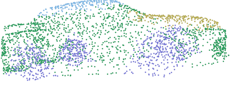
Fig. 6: PointNet part segmentation on ShapeNet dataset
- MNIST: This is the famous handwritten digit recognition. Althought being an image dataset, this can be converted easily to a point cloud dataset. For this dataset, only classification is available.
Going beyond PointNet
The introduction of PointNet was a great step forward. It allows to use point clouds as input for deep learning. However by essence PointNet has a big limitation: it cannot capture local structure induced by the metric space points live in, therefore making it unlikely to learn fine grained patterns or to understand complex scenes. This is due to the max pooling operation which takes the full cloud as input to produce a global feature. So although solving the invariance to permutation issue discussed above, PointNet does not really tackle the problem related to the desertion of shape. To answer to this limitation, the same author published later at NIPS 2017 an improvement over PointNet called PointNet++[8]. The principle of PointNet++ is pretty simple: a PointNet network is applied recursively to a nested partitioning of the input point set. The approach is somehow similar to CNN with images. The first layer kernels see very local data (small receptive field), but the deeper the layer, the larger the receptive field.
In addition to PointNet++, there have been several recent development among which the interesting PointCNN[9]. Their approach is quite different. They propose to learn a transformation that would learn a canonical representation of the input points invariant to permutations. From there, standard convolution could be applied. As the authors precised, the invariance to permutations is far from perfect, but they still claim to achieve state of the art results on principal point cloud datasets.
References
[1] "VoxNet: a 3D convolutional neural network for real time object recognition", Maturana & Scherer
[2] " Multi-view convolutional neural network for 3D shape recognition", Su et al
[3]"Visualizing and understanding convolutional networks", Zeiler & Fergus
[5] "Deep sets: modeling permutation invariance", Fuchs & Wagstaff & Engelcke
[6] "PointNet: Deep Learning on Point Sets for 3D Classification and Segmentation", Qi et al
[7] "Spatial Network Transformer", Jadeberg et al
[8] "PointNet++: Deep hierarchical learning on point sets in a metric space", Qi et al
[9] "PointCNN: convolution on -transformed points", Li et al
Credit cover picture: ESA/Hubble & NASA

Categories
- Artificial Intelligence (1)
- Big Data (4)
- CNN (1)
- Deep Learning (2)
- Django (1)
- Industrial Automation (1)
- Industry 4.0 (1)
- Machine Learning (3)
- PostgreSQL (3)
- Python (4)
- Pytorch (1)
- Spark (1)

